PiSCES Algorithms
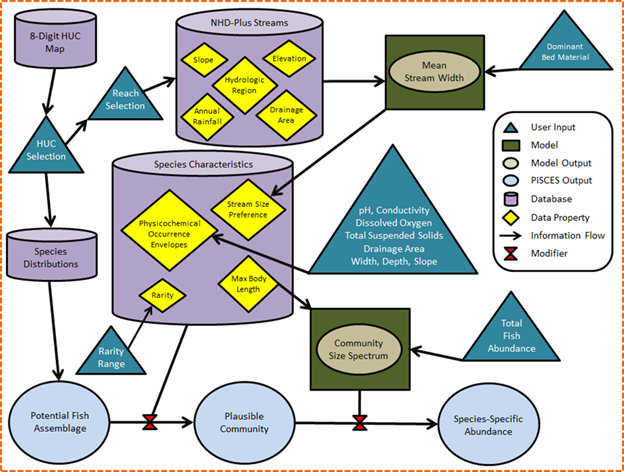
The PiSCES database incorporates environmental and biological information to predict fish species occurrence in watersheds of the continental U.S. Processing species and landscape data involves several steps.
To characterize stream size, the Peterson Guide defines lotic systems using a narrative term related to mean stream width:
- Headwater/Spring: 0-1 m
- Creek: 1-5 m
- Small River: 5-25 m
- Medium River: 25-50 m
- Large River: > 50 m
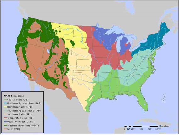
To calculate stream size for each river reach, bankfull width is derived using regional regression equations (Table 1, Figure 2) and converted to stream width under mean flow conditions by multiplying the bankfull width by 0.75 (Cassie, 2006).

Species Rarity descriptors (Page and Burr, 2011) were converted into a numeric scale:
- 1: Abundant
- 2: Abundant/Common
- 3: Common
- 4: Fairly Common
- 5: Common/Uncommon
- 6: Uncommon
- 7: Uncommon/Rare
- 8: Rare
- 9: Extremely Rare
- 10: Extinct
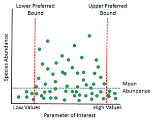
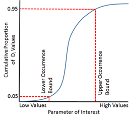
Our method for calculating occurrence envelopes (which hypothetically should be wider than preference bounds) can be described as follows:
- 1) Sort every site by a given parameter value (e.g., conductivity), smallest to largest
- 2) For each species, raise the recorded density at each site by an exponent ≥ 0. A value of 1 gives full weight to the measured densities, and the resulting envelopes will be influenced by sites where density of the species was highest. A value close to 0 transforms density data into presence/absence data, i.e., every site where the species was captured will be weighted equally.
- 3) For a species of interest, use the sorted site list to calculate a cumulative proportion (Pi) of the transformed
densities (Di) created in the previous step:

where n is the total number of sites in the dataset.
- 4) Identify the parameter values at the sites where Pi surpasses some threshold (e.g., the Lower Occurrence Envelope at 0.05; the Upper Occurrence Envelope at 0.95)
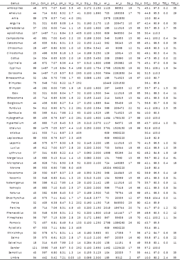
There were a total of 51 genera for which occurrence envelopes could be calculated using the mid-Atlantic EMAP and West Virginia REMAP data (Table 2). For most, we were able to calculate lower and upper bounds for the eight parameters we investigated. Missing values for cells in Table 2 arise because some parameters values were not recorded at some of the surveyed sites, so certain genus/parameter combinations dropped below a sample size of 5, stated earlier as our threshold for envelope calculation.
To fill in gaps in Table 2, we used envelope values from designated surrogate genera that shared ecological, morphological and/or physiological similarities to the genus with missing data (Table 3). We also used this approach to add four genera that were found in the EMAP/REMAP data, but for which no envelopes could be calculated because they were not found at more than 5 sites.

Table 4 shows the 10th and 90th percentiles of the eight investigated parameters from the 795 EMAP/REMAP survey sites. These were used to re-formulate the genera occurrence envelopes given in Table 2 based on a genus’ interpreted intolerance to extreme values of each parameter. For example, the 10th percentile of specific conductance across all examined sites was 45 µS/cm. In the second column of Table 2, each genus with a specific conductance lower bound less than 45 would be defined as “insensitive” to low specific conductance, and its lower envelope bound would be instead set to the lowest value of specific conductance found in the dataset (given in parentheses). When filtering a potential fish assemblage using stream characteristics, PiSCES gives the user the option of using the originally-formulated envelopes shown in Table 2, or these sensitivity-adjusted envelopes, which are less restrictive and will result in larger potential communities.

There is variability in tolerance and habitat preferences between species of the same genus (Barbour et al. 1999, Page and Burr 2011), but this variability is generally not as great as between-genera variability, thus these derived envelopes can be informative. Being genus-specific, the envelopes are wider than what would be expected for individual species, which will lead PiSCES to predict the possibility of more species than would commonly be found in a routine fish survey.
We employ a relationship between the body size of an organism (maximum length) and its abundance in a community, called the community size spectrum (Sheldon et al. 1972; Pope and Knights 1982; Han and Straškraba 1998; Boicourt et al. 2004):
The user sets α, a tuning parameter (default = 1). Smaller α values lead to a flatter spectrum, where there are almost as many large fish as small ones. Larger α values produce a steeper decline in abundance with increasing size, as is often the case in heavily exploited fisheries (Duplisea and Castonguay 2006). We suggest keeping this parameter between 0.5 and 2.0.
Table 5 shows how this approach works for a hypothetical community of seven fish species ranging in length from 10 to 60cm, with α = 1.5. The second column is log2Abundance. Column three is the anti-base2 logarithm (2^) of these values, and column four is each abundance divided by the sum of column three, so the values in Column 4 sum to 1. This relative abundance for each species is then multiplied by the user-specified total abundance (1,500 in this example) to provide an estimate of the absolute number of individuals of each species in the reach (column five).

For a subset of species in the PiSCES database, sensitivity to watershed disturbance and stream siltation were added using information in Barbour et al. (1999). This tolerance parameter is available as an assemblage filter in the PiSCES GUI. Species are categorized as Intolerant, Moderately Tolerant, or Tolerant.
The user can sort the PiSCES database to show groups of species that share evolutionary commonality (essentially corresponding to taxonomic families). The finalized PiSCES database contains information on 1015 fish species representing 200 genera. Table 6 shows categorization of the 49 groups in terms of sport fishes, non-game fishes, subsistence species, and those entirely exotic to the US. Note that some groups can be found in more than one column, and a group was classified according to the majority of the species comprising that group.

PiSCES also has the following ancillary information for each species in its database:
- Origin: Native to US or Introduced
- Human Use: Sport Fish, Non-Game, Subsistence
- Typical Systems Occupied: Caves, Springs, Headwaters, Creeks, Small Rivers, Medium River, Large Rivers, Lakes/Impoundments/Ponds/Canals/Ditches, Swamp/Marsh/Bayou, Coastal/Ocean
- Preferred Lotic Habitat: Riffles, Runs/Flowing Pools, Pools/Backwaters
- Preferred Location within the System: Benthic, Surface, Nearshore/Littoral, Pelagic
- Preferred Substrate: Mud/Silt/Detritus, Sand, Gravel, Rocks/Rubble/Boulders, Vegetation, Woody Debris/Brush
- Other Preferred Water Characteristics: Clear, Turbid, Warm, Cool, Cold, Lowland (low gradient), Upland (high gradient)
These descriptors were taken from information in Page and Burr (2011), NatureServe.com, and FishBase.org. Information on subsistence species was found in Kappen et al. (2012). For most fish groups, species whose maximum body size was over 25cm were considered sport fishes unless their rarity measure was 7 or greater. For Salmonids, this threshold was 20cm, and for Sunfish and Black Bass, the threshold was 15cm. Species under these thresholds were designated as non-game.
In summarizing PiSCES development outcomes and the introductory discussion on motivation, design, and intended use, three major benefits are derived from its final design and functionality. In stand-alone mode, PISCES allows users to develop reasonably reliable estimates of fish communities in lotic systems across the US. This functionality has numerous applications to serve a multitude of current assessment programs and research endeavors. Secondly, within an integrated environmental modeling framework (Johnston et al. 2011), PiSCES provides a service necessary to perform hydroecological assessments which link mechanistic hydrology models with ecological models to achieve prediction goals. Finally, PiSCES' general flexibility allows users to modify a community “best estimate” based on additional, waterbody-specific data. This functionality, established as an important design requirement, enhances the capabilities of both standalone use and integrated modeling applications for which it was created.